Forget about credit assignment in long-horizon agentic post-training

TL;DR

Evolution Strategies (ES) is a scalable zeroth-order alternative to policy-gradient (PG) RL for agentic post-training:

• ES (surprisingly) does not suffer from the curse of dimensionality when finetuning billion-parameter LLMs (Qiu et al. 2026, Liang et al. 2026).
• PG suffers from the curse of horizon: every generated token enters its gradient, so long agentic tasks need heavy credit-assignment engineering (TMax).
• On a synthetic task, PG wins at short horizons and ES wins at long horizons (in terms of sample efficiency). On 21 real tasks, PG’s lead shrinks as the effective horizon grows: current benchmarks sit at the start of the regime where ES begins to see an advantage.
• In preliminary experiments, fine-tuning Qwen3.5-4B with ES already achieves open-source SOTA performance on TBench!

So freaking simple, embarrassingly parallelizable, no credit assignment, no hacky tuning. We think it’s time to revisit zeroth-order methods for long-horizon agents.

Why ask this now

Fashion is a cycle; zeroth-order (weight-space) methods are making a comeback. Sometimes, simple methods just work, and surprisingly well at that (another bitter lesson yet). Policy-gradient-based methods (PG) like GRPO have dominated RL fine-tuning, but they struggle on long agentic tasks with issues like credit assignment over long rollouts, training instability, sensitivity to hyperparameters, etc. Recently, ES has been shown to work for finetuning billion-parameter models, and its performance has been shown to be comparable to that of SOTA PG methods. But if the performance is roughly similar, it is unclear what the key advantage of such zeroth-order methods is, especially considering the fact that in some cases they can be less sample efficient.

In this blog post, we aim to revisit the older topics of discussion related to ES and PG, particularly in light of comparing the two methods in their exploration currency (weight-space exploration vs. action-space exploration) and the tradeoff in their variances in gradient estimation, to determine in which regime one surpasses the other. Not to jump the gun, but it actually turns out that ES has many desirable qualities for finetuning on long-horizon tasks. We build on the following observations:

• Long-horizon agents are hard for PG. Tmax, T1 and TRACE each needed extra engineering (masking, actor-critic, per-action credit) to make PG work on Terminal-Bench-style tasks.
• Under terminal credit, every generated token enters the PG gradient, including tokens that do not affect the reward; we refer to this as the “curse-of-horizon.”
• ES at Scale (Qiu et al., 2026) showed ES can fine-tune 7B models, with mixed results against RL, and follow-up work (Liang et al., 2026) posits that the fact that ES can work in such high dimensionality indicates a lack of the traditional “curse-of-dimensionality.”
• The fact that ES bypasses the need for credit assignment, hence avoiding the curse of horizon, and that it does not suffer from the dimensionality curse makes it a stellar candidate for long-horizon agentic post-training.

We break down the theory and show concrete results in support of this thesis next.

Parameter-space vs. action-space exploration

Let’s start by revisiting algos to gain some theoretical intuition behind ES and PG. Assume that you have some underlying reward landscape that you want to hill-climb on. The reward landscape is jagged, and you have two viable options for approximating the gradient (or direction(s) that improve(s) reward in general; it doesn’t have to be the precise gradient), as illustrated in Figure 1:

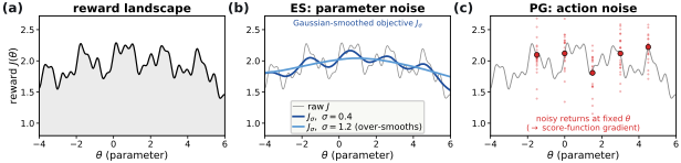
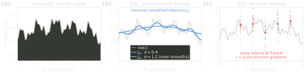
Figure 1: Parameter-space vs. action-space exploration. (a) A jagged reward landscape $J(\theta)$. (b) ES perturbs the weights, which amounts to climbing a Gaussian-smoothed version of the landscape, $J_\sigma$ (too large a σ over-smooths it). (c) PG keeps the weights fixed and samples actions, which gives noisy returns at a fixed θ.

1) evolution strategies (ES): you perturb the weights (isotropic Gaussian noise, full-rank or low-rank) N times, which forms a “population,” compute the reward corresponding to each perturbed candidate, and perform a weighted average of the perturbations by the outcome rewards to form an update step (an estimate of the gradient). Here is the math:

$$\hat g_\mathrm{ES} = \frac{1}{N\sigma}\sum_{i=1}^{N} R(\theta + \sigma\varepsilon_i)\,\varepsilon_i, \qquad \varepsilon_i \sim \mathcal{N}(0, I_D)$$

where θ are the model weights, σ is the perturbation scale, and $R(\theta + \sigma\varepsilon_i)$ is the outcome reward of the i-th perturbed model.

2) policy gradient (PG): you sample a trajectory (or a bunch of them), and compute the gradient of the output tokens’ log probabilities, weighted by their advantages. Here is the math:

$$\hat g_\mathrm{PG} = \frac{1}{G}\sum_{j=1}^{G}\sum_{t=1}^{T} \hat A_{j,t}\,\nabla_\theta \log \pi_\theta(a_{j,t} \mid s_{j,t}), \qquad a_j = (a_{j,1},\dots,a_{j,T}) \sim \pi_\theta$$

where $a_j$ is the j-th trajectory sampled from the current policy $\pi_\theta$ (with the weights held fixed), G is the number of sampled trajectories, T is the number of generated tokens, and $\hat A_{j,t}$ is the advantage of token t in trajectory j. With an outcome reward (e.g. GRPO), every token in a trajectory gets the same advantage, i.e. the trajectory’s reward minus the group-mean reward.

Now if you treat both methods as estimators of one underlying true gradient, $g^*$ (see below), that converge in expectation (an approximation we will go along with here for the sake of further analysis), then the bulk of the workload shifts to analyzing the variances of the two estimators. In particular, we are interested in how the two variances scale wrt different properties of the tasks.

$$g^* = \nabla_\theta J(\theta), \qquad \mathbb{E}\big[\hat g_\mathrm{ES}\big] = \nabla_\theta J_\sigma(\theta) \xrightarrow{\ \sigma \to 0\ } g^*, \qquad \mathbb{E}\big[\hat g_\mathrm{PG}\big] = g^*$$

where $J(\theta)$ is the expected reward and $J_\sigma$ is its Gaussian-smoothed version (Figure 1b).

Why variance analysis

If treated as gradient estimators, variances of the methods essentially dictate the sample efficiency/convergence speed of the learning methods. It’s about the signal-to-noise ratio of the learning methods. Assuming the same optimum is attainable by both methods (assume this for now, but it’s actually generally not true lol), the variance determines which method is cheaper.

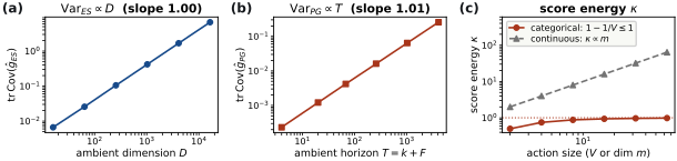
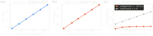
Figure 2: The naive curses. (a) ES variance grows linearly with the parameter count D. (b) PG variance grows linearly with the number of generated tokens T. (c) The per-token noise of PG (score energy κ) stays below 1 for a categorical policy like an LLM, whatever the vocabulary size, but grows with the action dimension for continuous actions.

Naively, ES variance grows with parameter count and PG variance grows with sequence length (Figure 2):

$$\text{ES cost} \propto D, \qquad \text{PG cost} \propto T$$

To put it quite plainly, ES is expected to suffer from the curse of dimensionality while PG suffers from the curse of horizon. However, in practice, this is more nuanced. In fact, only noise injected along directions that change the reward slows learning, so both costs shrink to effective counts.

Previously, it was long thought that because of the curse of dimensionality, there is no hope of applying ES to tune LLMs at the billion-parameter level. However, this has been shown not to be true by ES-at-scale and a series of follow-up works (Sarkar et al., 2026; Liang et al., 2026; Schweighofer et al., 2026; Gan et al., 2026). Indeed, many of these works point to one reality, which is that finetuning LLMs is surprisingly simple and low-dimensional, and practically many methods can work. So concern for the curse of dimensionality is out the door, great!

However, things are not looking so rosy for the horizon curse in the case of PG. Even though a reward-irrelevant token adds PG noise only if it gets credit from the reward and its gradient overlaps the reward-relevant directions, in an LLM the overlap is almost to be expected since we generate autoregressively. Moreover, the effective horizon is further determined by how well you can do credit assignment, which becomes increasingly difficult as your horizon grows, unboundedly so for some of the modern agentic tasks.

A combination lock to pull the two costs apart

To pull the two costs (dimension and horizon) apart controllably, we design a toy multi-combo lock task. The task is very simple: it is essentially a (non-autoregressive) $k$-digit multi-combination lock with $T = k + F$ slots. The policy network (here an MLP that takes in a skill-specific position code and outputs logits over $V$-vocab) just has to memorize $r$ length-$k$ sequences; the remaining F slots are filler (distractor) tokens that do not affect the outcome rewards. The task is illustrated below:

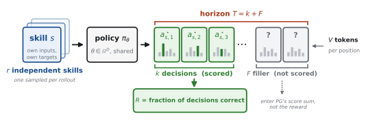
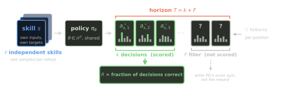
Figure 3: The multi-skill combination lock. Each rollout samples one of r independent skills, and a policy $\pi_\theta$ with shared weights emits T = k + F tokens from a vocabulary of size V. The reward is the fraction of the k scored decisions that are correct, while the F filler tokens are not scored but still enter the PG gradient.

Essentially, by varying $r$ (number of combos), $k$ (number of scored slots) and $F$ (number of filler slots), we get to controllably vary the effective dimension and horizon, which allows us to identify regimes under which one method dominates the other in cost. The outcome is quite clean:

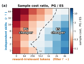
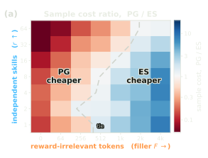
Figure 4: Which method is cheaper across the number of skills r and the filler length F, with both methods tuned in every cell. Color shows the ratio of the sample costs of PG and ES (red: PG cheaper, blue: ES cheaper), and the dashed line marks where the two tie. The tie moves to longer horizons as the number of skills grows.

Here, we tune both methods in every setting and record the number of samples each method needs to reach 90% performance. PG is cheaper at short horizons and ES is cheaper at longer horizons. The crossover between the costs of the two methods is determined by a bunch of factors, but, to put it plainly, can be summarized by $D_\text{eff}$ and $T_\text{eff}$:

$$\text{ES cost} \propto D_\mathrm{eff} = r\,k, \qquad \text{PG cost} \propto T_\mathrm{eff} = k + \gamma\,\beta\,F$$

where γ comes from weight sharing, and β from credit assignment.

The intuition behind the γ and the β factors is the following: γ measures how much the representations of the filler tokens and the decision tokens overlap, and β measures how much the filler tokens get credited (that is, misattributed).

	γ → 0 (no overlap)	γ > 0 (shared weights)
β → 0 (per-token credit)	free	free
β ≈ 1 (terminal credit)	free	paid for

So the horizon tax incurred by the filler tokens is actually discounted by both factors above. Note that this is a simplified expression assuming each filler position contributes uniformly, which is most definitely not the case in general. However, the general-case analysis is of a similar spirit and does not change the conclusions. We also left out a bunch of detailed analysis for the sake of keeping the blog post simple, so interested readers can find out more in our paper (link coming soon!).

Where real tasks sit on the horizon axis

Now the real question is where the real tasks sit on this dimension v. horizon phase diagram, and whether their relative positions predict their ES-PG head-to-head performance comparison. To answer it, we needed to approximately measure the effective dimension and effective horizon on these tasks with respect to some base models.

Measuring both quantities reliably turns out to be tricky, especially the effective dimensionality. One measure is to approximate the effective dimension by the effective rank of the token log-likelihood gradients on the reference solutions (written by humans). This approach, however, picks up mostly on the stylistic mismatch between the base model and the reference solutions. Sparing the details, we therefore only show the horizon of these tasks (panel a below) and the relative performance diff between ES- and PG-tuned solutions on these tasks vs. their task horizons (panel b).

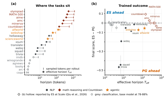
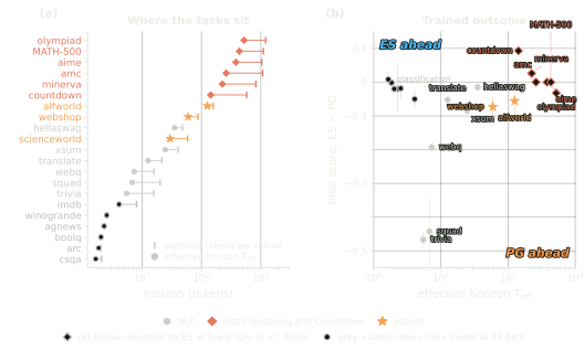
Figure 5: Real tasks on the horizon axis. (a) Sampled tokens per rollout (tick) and effective horizon $T_\text{eff}$ (marker) of each task. (b) Final score of ES minus that of PG against $T_\text{eff}$. Filled markers are our own tuned head-to-heads, and hollow ones are reported by ES at Scale. PG’s lead shrinks as the effective horizon grows.

We measured the effective horizon of 21 tasks in the setup each one is trained in. The task set includes 12 NLP tasks, 3 agentic environments (ALFWorld, WebShop, ScienceWorld), plus Countdown and five math benchmarks from ES at Scale. All use 7B Qwen2.5 models (instruct or math). One catch here is that the Qwen2.5 7B models cannot (or only very, very rarely) solve any of the TBench tasks, so we leave TBench out of Figure 5 and instead compare ES and PG on TBench with Qwen3.5-4B. Here is the result for TBench (very preliminary, more details to come):

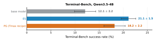
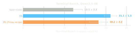
Figure 6: Terminal-Bench success rate of Qwen3.5-4B before training, after ES fine-tuning, and after PG training with the Tmax recipe (mean with error bars).

Here is how the horizon measurement works: we count each sampled token by how much of its gradient lies in the directions that change the reward, which gives the effective horizon (the marker, a lower bound); the raw generated token count sets the upper cap (the tick). Note that this measure is also approximate and is strongly coupled to the base model performance on the particular task, so we use it to rank tasks, not to draw a hard boundary of when one method surpasses the other.

As panel a shows, classification tasks (imdb, winogrande, agnews, boolq, arc, and csqa) typically require a few (effective) tokens, other NLP (trivia, squad, webq, translate, xsum, hellaswag) up to a few dozen, action-only agents (scienceworld, webshop, alfworld) up to about a hundred, and math a few hundred (countdown, minerva, amc, aime, math500, olympiad). Notably, even the longest of them reach only the low end of the crossover range, as shown by panel b, which suggests that the mixed ES-vs-PG (GRPO/PPO) results reported previously are due to these benchmarks having effective horizons at the onset of true ES advantage. We hence expect ES to have more advantage in the longer-horizon regimes.

When to go for ES

Other reasons that you might consider ES

• It uses only forward passes, stores no activations, and runs perturbed models in parallel on inference engines.
• It also repairs confident wrong decisions that PG’s gradient cannot fix (the lock-repair appendix).
• It needs no credit assignment or messy HP tuning.

These properties make ES a promising candidate for post-training in the agentic era.

Links and credits

Qiyao Liang, Kajetan Schweighofer, Xin Qiu and Risto Miikkulainen (Cognizant AI Lab). A preliminary version of this work appeared at the SciFM workshop (best paper runner-up) at COLM 2026. For more details and citations, please refer to our manuscript (coming soon).

To cite this blog post in the meantime:

@misc{liang2026forget,
  title  = {Forget about credit assignment in long-horizon agentic post-training},
  author = {Liang, Qiyao and Schweighofer, Kajetan and Qiu, Xin and Miikkulainen, Risto},
  year   = {2026},
  month  = nov,
  note   = {Blog post}
}

References

• Gan, Y., & Isola, P. (2026). Neural Thickets: Diverse Task Experts Are Dense Around Pretrained Weights. arXiv:2603.12228
• Ivison, H., Yin, J. O., Shao, R., Xiao, T., Lambert, N., & Hajishirzi, H. (2026). Tmax: A Simple Recipe for Terminal Agents. arXiv:2606.23321
• Liang, Q., Song, J., Liu, Y., Gore, J., Fiete, I., Miikkulainen, R., & Qiu, X. (2026). The Blessing of Dimensionality in LLM Fine-tuning: A Variance-Curvature Perspective. arXiv:2602.00170
• Merrill, M. A., Shaw, A. G., Carlini, N., Li, B., Raj, H., et al. (2026). Terminal-Bench: Benchmarking Agents on Hard, Realistic Tasks in Command Line Interfaces. ICLR 2026. arXiv:2601.11868
• Qiu, X., Gan, Y., Hayes, C. F., Liang, Q., Xu, Y., Dailey, R., Meyerson, E., Hodjat, B., & Miikkulainen, R. (2026). Evolution Strategies at Scale: LLM Fine-Tuning Beyond Reinforcement Learning. ICML 2026. arXiv:2509.24372
• Sarkar et al. (2026). Evolution Strategies at the Hyperscale. ICML 2026. arXiv:2511.16652
• Schweighofer, K., Hayes, C. F., Dailey, R., Miikkulainen, R., & Qiu, X. (2026). Overcoming Forgetting in LLM Fine-Tuning with Evolution Strategies. arXiv:2605.30148
• Takehi, R., Teoh, J., Zhang, A., & Khattab, O. (2026). Sparks of Weight-Space Programming: LLMs can natively read & write neural network weights. Blog post
• Tao, L., Peng, B., Yao, W., Ge, T., Cheng, H., Wang, M. H., Gao, J., & Li, S. (2026). TRACE: Turn-level Reward Assignment via Credit Estimation for Long-Horizon Agents. arXiv:2607.13988
• Yang, J., Shi, Y., Li, Z., Wang, R., Li, Z., Mi, H., & Liang, L. (2026). T1: Terminal Agent Reinforcement Learning for Long-Horizon Tasks. arXiv:2609.11042
• Zhu, D., et al. (2026). EdgeBench: Unveiling Scaling Laws of Learning from Real-World Environments. arXiv:2607.05155

Appendix

Lock-and-repair mechanism of ES

So one really interesting phenomenon that we noticed was the decision commitment of PG vs. ES. PG methods are known to suffer from mode collapse, which means they lock into policies that emit (wrong) decision tokens confidently and consistently such that the diversity of output is murdered and there is little chance of getting unstuck. On the synthetic task, where we are able to systematically vary the horizon length and can cheaply afford to tune the HPs of each method, we found that this locking phenomenon is increasingly prominent for task settings with longer horizon (higher F) and higher dimension (higher r). The learning dynamics (one color per skill) are plotted below for all PG settings, along with their ES counterparts (ES only has one row because it does not care about the horizon length).

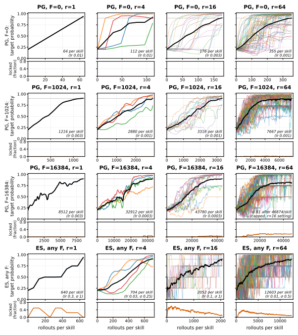
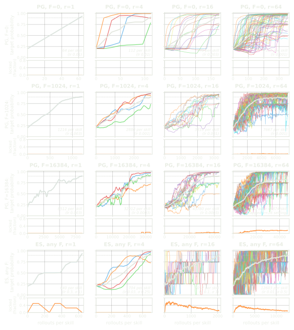
Figure 7: Learning dynamics on the combination lock, with both methods tuned in every setting. The top three rows are PG at increasing filler length F, and the bottom row is ES, which does not depend on F. Columns increase the number of skills r. In each panel, thin colored lines are individual skills, the thick line is their mean, and the dotted line marks the 0.9 target. The orange strip below each panel shows the fraction of decisions locked onto a wrong token. PG’s locked fraction grows with F and r and stays there, while ES’s rises early and then decays as it unlocks them.

The only defense for PG in this case is actually to reduce the step size, to slow down the rate of accumulating these locked decision tokens, which inevitably slows down the progress of learning. ES, on the other hand, has the ability to correct itself over the course of learning (as shown by the orange panels, which track the fraction of locked tokens over training), which makes it more robust to the HP settings. This indicates that exploration in parameter space vs. action space can allow the two methods to discover fundamentally different solutions. To circle back to the discussion in the main text, variance comparisons only matter for the cost comparison of the methods, but the exploration mechanisms matter for determining the final attainable performance outcomes.